Further Tutorial: Selecting a Galaxy Sample from IllustrisTNG#
This tutorial demonstrates how to load group catalog of a specific snapshot from the TNG50-1 simulation using the illustris_python API, calculate physical properties, and filter galaxies based on mass and SFR. For this example, we will select a sample of massive, quiescent galaxies at z~1.5 (snapshot number=40).
import os, sys
import numpy as np
import matplotlib.pyplot as plt
import illustris_python as il
We define the path to the simulation data and load the subhalo (galaxy) catalog for a specific snapshot (redshift). We point illustris_python at the simulation output directory and load all subhalo fields for the chosen snapshot.
Tip: Change snap_number to select a different redshift. Use the TNG snapshot table to find the snapshot index that corresponds to your target redshift. Download group catalogs from this link and follow instruction at this link for instructions on storing the data.
# Path to the TNG50-1 simulation output on the local disk
basePath = '/Volumes/disk4tb/data/TNG/TNG50-1/output'

# Snapshot number 40 corresponds to a specific redshift (e.g., z ≈ 1.5)
snap_number = 40

# Load the subhalo (galaxy) catalog from the groupcat
subhalos = il.groupcat.loadSubhalos(basePath, snap_number)
In this example, we pull three key fields from the catalog and convert them to physical units. The Hubble parameter h = 0.6774 converts the raw simulation mass unit (10^10 M_sun / h) to solar masses. More fields from the catalog can be seen at this link.
# Hubble parameter for TNG simulations
h = 0.6774

# Extract stellar mass within twice the stellar half-mass radius (index 4 = stars)
# Convert from 1e10 M_sun/h to M_sun
mstar_2re = subhalos['SubhaloMassInRadType'][:,4] * 1e+10 / h

# Extract the Star Formation Rate (SFR) and the half-mass radius
sfr_2re = subhalos['SubhaloSFRinRad']

# get half stellar mass radius and convert into kpc
from galsyn.simutils_tng import get_snap_z
api_key = "7ae4d3ea8a7c808a0932e62abc69dde4"
snap_z = get_snap_z(snap_number, sim='TNG50-1', api_key=api_key)
snap_a = 1.0/(1.0 + snap_z)
halfmass_rad = subhalos['SubhaloHalfmassRadType'][:,4] * snap_a / h  # in kpc

# Print the total number of subhalos found in this snapshot
snap_ngals = len(mstar_2re)
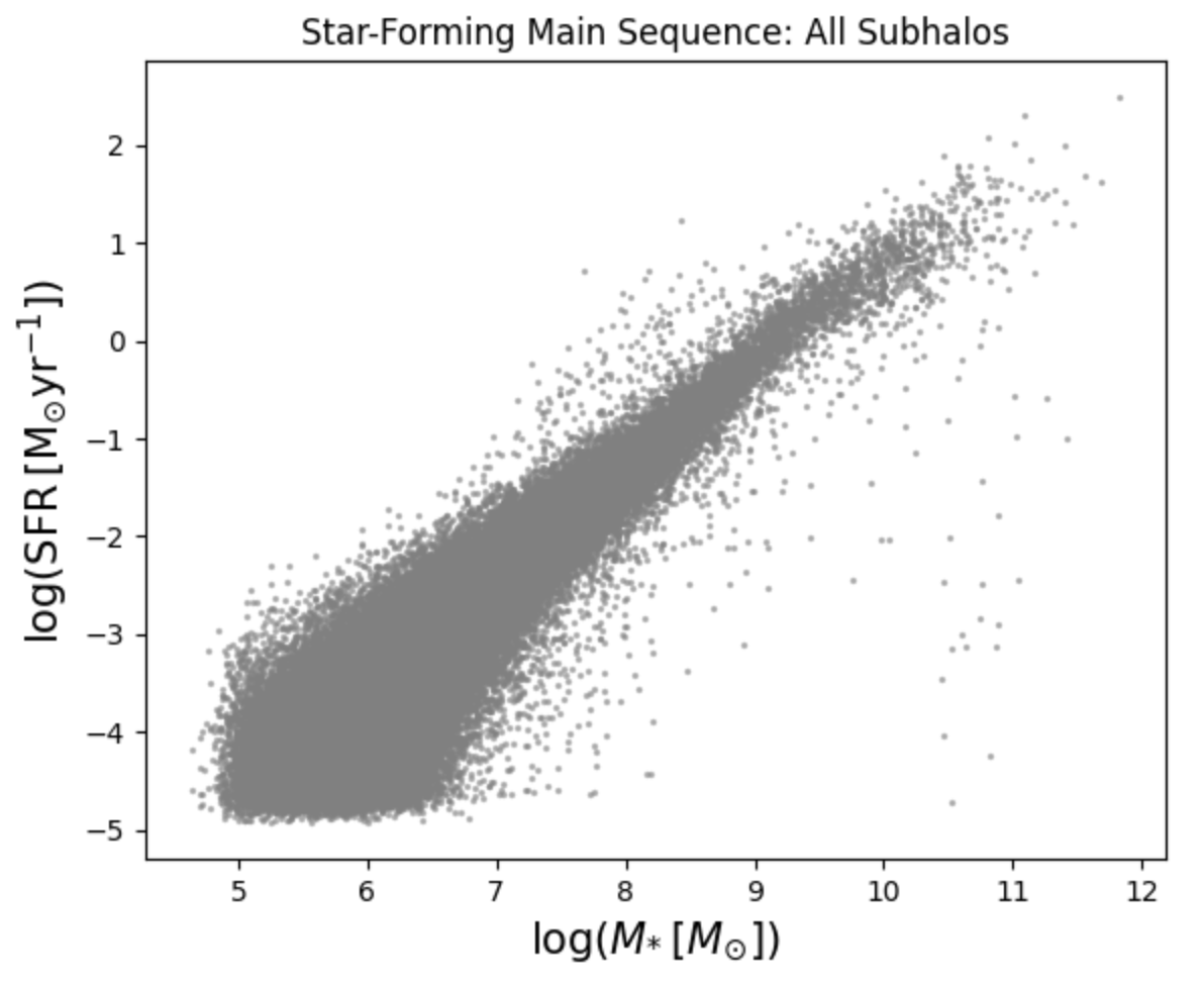
We plot log(SFR) vs. log(M_star) for every subhalo in the snapshot. This diagnostic plot reveals the full galaxy population, including the star-forming main sequence and the cloud of passive/quenched objects below it.
fig, ax = plt.subplots(figsize=(6, 5))

# All subhalos plotted in grey with low opacity
ax.scatter(np.log10(mstar_2re), np.log10(sfr_2re),
        s=2, color='gray', alpha=0.5)

ax.set_xlabel(r'$\log(M_{*}\,[M_{\odot}])$', fontsize=15)
ax.set_ylabel(r'$\log(\rm{SFR}\,[M_{\odot}\rm{yr}^{-1}])$', fontsize=15)
ax.set_title('Star-Forming Main Sequence: All Subhalos')

plt.tight_layout()
plt.show()
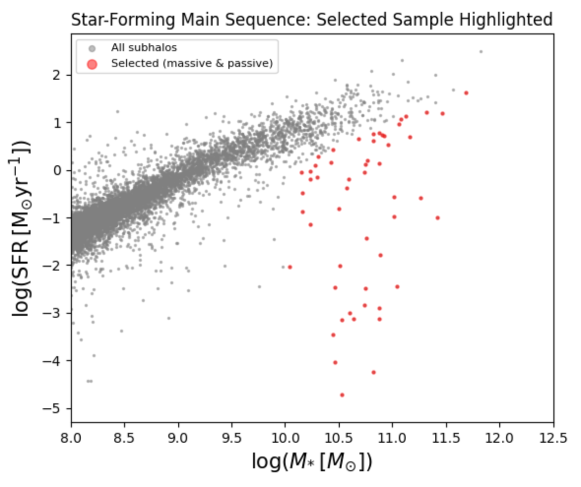
In this example, we select subhalos that are massive and passive (quiescent). The selected galaxies are then overplotted in red on the star-forming main sequence diagram.
# Selection mask: massive (log M* > 10) AND passive (sSFR < 10^-10 / yr)
idx_select = np.where(
    (np.log10(mstar_2re) > 10.0) &                               # mass cut
    (np.log10(sfr_2re) - np.log10(mstar_2re) < -10.0)           # sSFR cut
)[0]

print('Number of selected galaxies: %d' % len(idx_select))

# --- Diagnostic plot ---
fig, ax = plt.subplots(figsize=(6, 5))

ax.set_xlim(8.0, 12.5)

# Background: all subhalos (grey)
ax.scatter(np.log10(mstar_2re), np.log10(sfr_2re),
        s=2, color='gray', alpha=0.5, label='All subhalos')

# Foreground: selected passive massive galaxies (red)
ax.scatter(np.log10(mstar_2re[idx_select]), np.log10(sfr_2re[idx_select]),
        s=5, color='red', alpha=0.5, label='Selected (massive & passive)')

ax.set_xlabel(r'$\log(M_{*}\,[M_{\odot}])$', fontsize=15)
ax.set_ylabel(r'$\log(\rm{SFR}\,[M_{\odot}\rm{yr}^{-1}])$', fontsize=15)
ax.set_title('Star-Forming Main Sequence: Selected Sample Highlighted')
ax.legend(markerscale=3, fontsize=8)

plt.tight_layout()
plt.show()
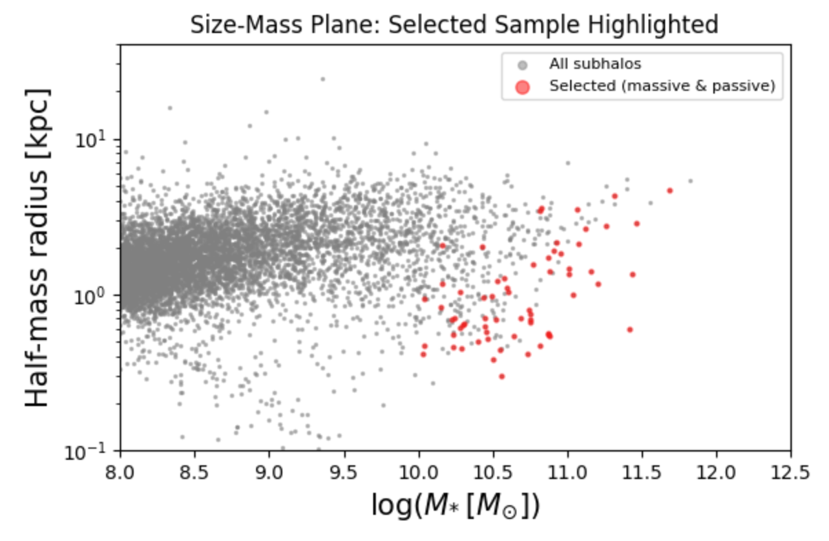
We plot the stellar half-mass radius against log(M_star) for all subhalos and highlight the selected passive sample in red.
fig, ax = plt.subplots(figsize=(6, 4))

ax.set_xlim(8.0, 12.5)
ax.set_ylim(0.1, 40.0)
ax.set_yscale('log')   # log y-axis to capture the full size dynamic range

# Background: all subhalos (grey)
ax.scatter(np.log10(mstar_2re), halfmass_rad,
        s=2, color='gray', alpha=0.5, label='All subhalos')

# Foreground: selected massive passive galaxies (red)
ax.scatter(np.log10(mstar_2re[idx_select]), halfmass_rad[idx_select],
        s=5, color='red', alpha=0.5, label='Selected (massive & passive)')

ax.set_xlabel(r'$\log(M_{*}\,[M_{\odot}])$', fontsize=15)
ax.set_ylabel('Half-mass radius [kpc]', fontsize=15)
ax.set_title('Size-Mass Plane: Selected Sample Highlighted')
ax.legend(markerscale=3, fontsize=8)

plt.tight_layout()
plt.show()
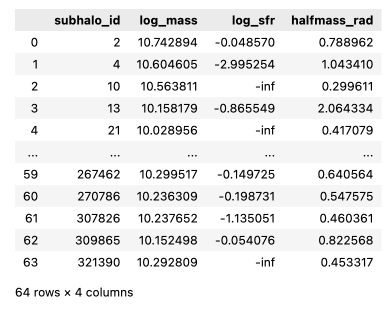
Show list of selected galaxies in a table.
import pandas as pd

# Accumulate one record per selected galaxy
selected_galaxies = []
for idx in idx_select:
    # Use a descriptive variable name to avoid shadowing the built-in 'dict'
    entry = {
        'subhalo_id':   int(idx),                      # integer catalog row index
        'log_mass':     np.log10(mstar_2re[idx]),      # log10 stellar mass  [M_sun]
        'log_sfr':      np.log10(sfr_2re[idx]),        # log10 SFR  [M_sun/yr]  (-inf if SFR=0)
        'halfmass_rad': halfmass_rad[idx],             # stellar half-mass radius
    }
    selected_galaxies.append(entry)

# Convert the list of dicts to a Pandas DataFrame
df = pd.DataFrame(selected_galaxies)
df