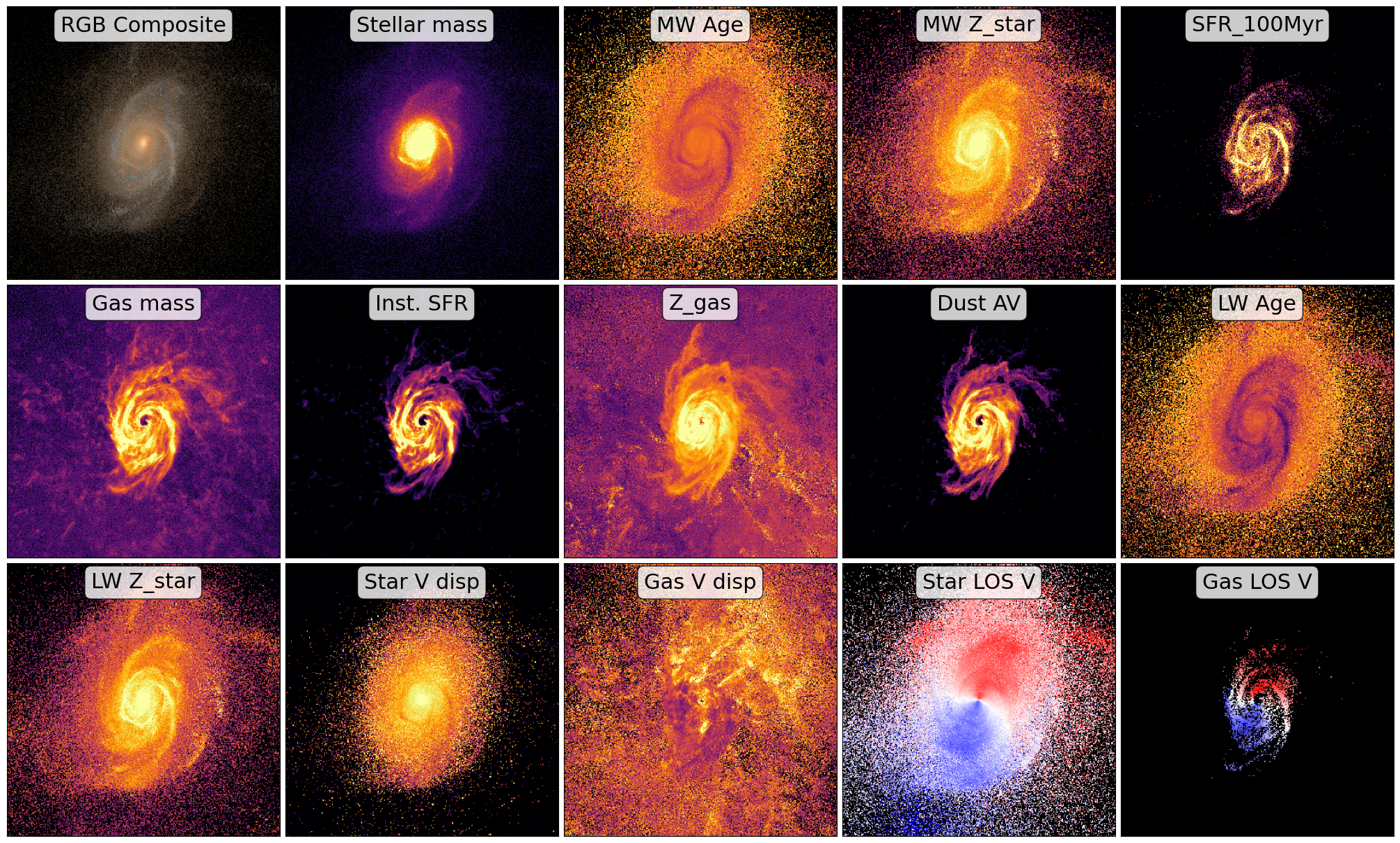
Analyzing Spatially Resolved Physical Property Maps#
After running the synthesis process, GalSyn produces a comprehensive FITS file containing synthetic imaging, IFU data cubes, and extensive set of physical property maps. The script below demonstrates how to visualize these spatially resolved phsyical property maps.
import numpy as np
import matplotlib.pyplot as plt
import matplotlib.cm as cm
from astropy.io import fits
from astropy.visualization import simple_norm, make_lupton_rgb

# Input synthetic data cube
fits_filename = 'galsyn_39_107965_specphoto.fits'

# Your specific HDU names and labels
hdu_names = [
    'STARS_MASS', 'MW_AGE', 'STARS_MW_ZSOL', 'SFR_100MYR', 'GAS_MASS', 'SFR_INST',
    'GAS_MW_ZSOL', 'DUST_MEAN_AV', 'LW_AGE_DUST', 'LW_ZSOL_DUST',
    'STARS_VEL_DISP_LOS', 'GAS_VEL_DISP_LOS', 'LW_VEL_LOS_DUST',
    'LW_VEL_LOS_NEBULAR'
]

prop_labels = {
    'STARS_MASS':'Stellar mass', 'MW_AGE': 'MW Age', 'STARS_MW_ZSOL': 'MW Z_star',
    'SFR_100MYR': 'SFR_100Myr', 'GAS_MASS': 'Gas mass', 'SFR_INST': 'Inst. SFR',
    'GAS_MW_ZSOL': 'Z_gas', 'DUST_MEAN_AV': 'Dust AV', 'LW_AGE_DUST': 'LW Age',
    'LW_ZSOL_DUST': 'LW Z_star', 'STARS_VEL_DISP_LOS': 'Star V disp',
    'GAS_VEL_DISP_LOS': 'Gas V disp', 'LW_VEL_LOS_DUST': 'Star LOS V',
    'LW_VEL_LOS_NEBULAR': 'Gas LOS V'
}

# RGB Filters from your example
rgb_fils = ['jwst_nircam_f115w', 'jwst_nircam_f150w', 'jwst_nircam_f200w']
rgb_factor = 3e+3

# Open the data cube
hdulist = fits.open(fits_filename)

# Calculate grid (Total = 1 RGB + all hdu_names)
num_plots = len(hdu_names) + 1
ncols = 5
nrows = (num_plots + ncols - 1) // ncols

fig, axes = plt.subplots(nrows, ncols, figsize=(4 * ncols, 4 * nrows), constrained_layout=True)
axes = axes.flatten()

# Panel 1: RGB image
ax_rgb = axes[0]
# Use the DUST_[FILTER] naming convention from your RGB example
r = hdulist[f'DUST_{rgb_fils[2].upper()}'].data * rgb_factor
g = hdulist[f'DUST_{rgb_fils[1].upper()}'].data * rgb_factor
b = hdulist[f'DUST_{rgb_fils[0].upper()}'].data * rgb_factor

rgb_image = make_lupton_rgb(r, g, b, stretch=20, Q=15)
ax_rgb.imshow(rgb_image, origin='lower')
ax_rgb.text(0.5, 0.93, "RGB Composite", transform=ax_rgb.transAxes,
            bbox=dict(boxstyle="round,pad=0.3", facecolor="white", alpha=0.8),
            verticalalignment='center', horizontalalignment='center', fontsize=22)
ax_rgb.set_xticks([])
ax_rgb.set_yticks([])

# Subsequent panels: physical property maps
for i, ext_name in enumerate(hdu_names):
    ax = axes[i + 1] # Offset by 1 to skip the RGB panel

    data = hdulist[ext_name].data

    # Inside your loop, before calling ax.imshow:
    if 'VEL_LOS' in ext_name:
        # 1. Create a mask for values that are exactly zero
        # (or very close to it, depending on your data)
        masked_data = np.ma.masked_equal(data, 0.0)

        cmap = cm.get_cmap('bwr').copy()
        cmap.set_bad(color='black')

        im = ax.imshow(masked_data, origin='lower', cmap=cmap, vmin=-300, vmax=300)

    else:
        cmap = cm.get_cmap('inferno').copy()
        cmap.set_bad(color='black')
        norm = simple_norm(data, 'sqrt', percent=98.0)
        im = ax.imshow(data, norm=norm, origin='lower', cmap=cmap)

    # Labels
    title_label = prop_labels.get(ext_name, ext_name)
    ax.text(0.5, 0.93, title_label, transform=ax.transAxes,
            bbox=dict(boxstyle="round,pad=0.3", facecolor="white", alpha=0.8),
            verticalalignment='center', horizontalalignment='center', fontsize=22)

    ax.set_xticks([])
    ax.set_yticks([])

hdulist.close()

plt.show()