Generating Idealized Synthetic Data Cubes

With all the preparatory steps completed, we can now initialize the GalaxySynthesizer class and run the synthesis process. To generate synthetic data cubes using GalaxySynthesizer, we need the filters and their transmission curves that are set up previously in Setting up Filter Transmission Curves.

Generating idealized imaging data cubes

The following script demonstrates the generation of imaging data cube. We will use the line-of-sight (LOS) dust-attenuation modeling method for estimating the dust optical depth for each star particle light. For the dust attenuation curve, we will use the modified Calzetti law (option 0) with varying (i.e., adaptive) slope and bump amplitude depending on \(A_{V}\).

from galsyn import GalaxySynthesizer
from galsyn.simutils_tng import get_snap_z

# Your personal API key from the IllustrisTNG website
api_key = "your_api_key"

# Specify simulation parameters
sim = 'TNG50-1'         # The TNG simulation run
snap_number = 39        # The snapshot index (e.g., z ~ 1.5 in IllustrisTNG)
subhalo_id = 107965     # The subhalo ID

# Assign a redshift to the galaxy. This value can be arbitrary, provided it is reasonably close to the exact redshift of the snapshot index.
# In this example, we will fetch the precise redshift for the snapshot number using the TNG API.
z = get_snap_z(snap_number, api_key=api_key)
print ('Redshift: %lf' % z)

# Define the path for the standardized input file, generated using the script in Example 1
sim_file = f'sim_file_tng_{int(snap_number)}_{int(subhalo_id)}.hdf5'

gs = GalaxySynthesizer(sim_file, z=z, filters=filters, filter_transmission_path=filter_transmission_path)

gs.ssp_filepath = 'ssp_fsps_a100_z100_u10.hdf5'         # path to the FSPS SSP grids generated in Example 2
gs.ssp_interpolation_method = 'linear'

gs.dim_kpc = 90                # Image side length in kpc
gs.smoothing_length = 0.15     # Smoothing length of the simulation in kpc
gs.pix_arcsec = 0.03           # Output pixel scale in arcseconds

gs.flux_unit = 'MJy/sr'        # Desired unit for the output FITS file

gs.polar_angle_deg = 0.0       # Polar angle or inclination
gs.azimuth_angle_deg = 0.0     # azimuth angle or rotation in the xy-plane

# Dust attenuation modeling method
gs.dust_method = 'los'             # line-of-sight method

# modified Calzetti et al. (2000) with variable slope and Bump
gs.dust_law = 0

# Apply adaptive dust index based on AV-slope relation from Salim+18
from galsyn.dust import relation_AVslope
dict_AV_slope = relation_AVslope(model_name="salim18")
gs.dust_index = dict_AV_slope

# Apply adaptive Bump amplitude based on its relation with the dust index from Kriek & Conroy (2013)
from galsyn.dust import bump_amp_from_dust_index
bump_amp = bump_amp_from_dust_index(dict_AV_slope["dust_index"])
dict_AV_bump_amp = {'AV':dict_AV_slope["AV"], 'bump_amp':bump_amp}

# Apply fixed Bump width
gs.bump_dwave = 0.035

# For the dust scaling with redshift, we will use the dust optical depth normalization
# (as a function of redshift) from Vogelsberger et al. (2020)
from galsyn.dust import relation_AVslope, scale_dust_redshift_Vogelsberger20
dict_scale_dust_redshift0 = scale_dust_redshift_Vogelsberger20()
dict_scale_dust_redshift = {'z': dict_scale_dust_redshift0['z'], 'tau_dust': dict_scale_dust_redshift0['tau_dust']*1.6}
gs.scale_dust_redshift = dict_scale_dust_redshift

gs.dust_eta = 2.0                # Ratio of AV in birth clouds vs diffuse ISM
gs.dust_index_bc = -0.7          # Power-law slope for birth clouds

gs.ncpu = 5                      # number of CPU cores to use
gs.output_pixel_spectra = False  # Generate broadband images only (not including spectra)

gs.name_out_img = f'galsyn_{int(snap_number)}_{int(subhalo_id)}_photo.fits'

# Run the synthetis process
gs.run_synthesis()

Generating idealized imaging + spectroscopy data cubes

The following script demonstrates the generation of spectrophotometric data cube with line-of-sight dust-attenuation modeling method and the modified Calzetti dust law with a dynamic slope and bump strength that depends on \(A_{V}\).

from galsyn import GalaxySynthesizer
from galsyn.simutils_tng import get_snap_z

# Your personal API key from the IllustrisTNG website
api_key = "your_api_key"

# Specify simulation parameters
sim = 'TNG50-1'         # The TNG simulation run
snap_number = 39        # The snapshot index (e.g., z ~ 1.5 in IllustrisTNG)
subhalo_id = 107965     # The subhalo ID

# Assign a redshift to the galaxy. This value can be arbitrary, provided it is reasonably close to the exact redshift of the snapshot index.
# In this example, we will fetch the precise redshift for the snapshot number using the TNG API.
z = get_snap_z(snap_number, api_key=api_key)
print ('Redshift: %lf' % z)

# Define the path for the standardized input file, generated using the script in Example 1
sim_file = f'sim_file_tng_{int(snap_number)}_{int(subhalo_id)}.hdf5'

gs = GalaxySynthesizer(sim_file, z=z, filters=filters, filter_transmission_path=filter_transmission_path)

gs.ssp_filepath = 'ssp_fsps_a100_z100_u10.hdf5'         # path to the FSPS SSP grids generated in Example 2
gs.ssp_interpolation_method = 'linear'

gs.dim_kpc = 90                # Image side length in kpc
gs.smoothing_length = 0.15     # Smoothing length of the simulation in kpc
gs.pix_arcsec = 0.03           # Output pixel scale in arcseconds

gs.flux_unit = 'MJy/sr'        # Desired unit for the output FITS file

gs.polar_angle_deg = 0.0       # Polar angle or inclination
gs.azimuth_angle_deg = 0.0     # azimuth angle or rotation in the xy-plane

# Dust attenuation modeling method
gs.dust_method = 'los'             # line-of-sight method

# modified Calzetti et al. (2000) with variable slope and Bump
gs.dust_law = 0

# Apply adaptive dust index based on AV-slope relation from Salim+18
from galsyn.dust import relation_AVslope
dict_AV_slope = relation_AVslope(model_name="salim18")
gs.dust_index = dict_AV_slope

# Apply adaptive Bump amplitude based on its relation with the dust index from Kriek & Conroy (2013)
from galsyn.dust import bump_amp_from_dust_index
bump_amp = bump_amp_from_dust_index(dict_AV_slope["dust_index"])
dict_AV_bump_amp = {'AV':dict_AV_slope["AV"], 'bump_amp':bump_amp}

# Apply fixed Bump width
gs.bump_dwave = 0.035

# For the dust scaling with redshift, we will use the dust optical depth normalization
# (as a function of redshift) from Vogelsberger et al. (2020)
from galsyn.dust import relation_AVslope, scale_dust_redshift_Vogelsberger20
dict_scale_dust_redshift0 = scale_dust_redshift_Vogelsberger20()
dict_scale_dust_redshift = {'z': dict_scale_dust_redshift0['z'], 'tau_dust': dict_scale_dust_redshift0['tau_dust']*1.6}
gs.scale_dust_redshift = dict_scale_dust_redshift

gs.dust_eta = 2.0                # Ratio of AV in birth clouds vs diffuse ISM
gs.dust_index_bc = -0.7          # Power-law slope for birth clouds

gs.ncpu = 5                      # number of CPU cores to use

# Set up output spectra
# Wavelength range set here should be within the range set for the SSP grids in Example 2
# Wavelength incerement determines the number of wavelength grids in the IFS data and resulting file size
gs.output_pixel_spectra = True   # Include spectra
gs.rest_wave_min = 1000.0
gs.rest_wave_max = 30000.0
gs.rest_delta_wave = 5.0         # in Angstrom

gs.name_out_img = f'galsyn_{int(snap_number)}_{int(subhalo_id)}_specphoto.fits'

# Run the synthetis process
gs.run_synthesis()

Check the generated data cube

In the following scipt, we extract some images from the data cube, make RGB image, and show them in a plot.

from astropy.io import fits
import matplotlib.pyplot as plt
from astropy.visualization import simple_norm, make_lupton_rgb

cube = fits.open('galsyn_39_107965_specphoto.fits')

# Filter configuration
fils = ['hst_acs_f606w', 'hst_acs_f814w', 'hst_wfc3_ir_f160w', 'jwst_nircam_f150w',
        'jwst_nircam_f277w', 'jwst_nircam_f356w', 'jwst_nircam_f444w']
filnames = ['JWST/F606W', 'JWST/F814W', 'JWST/F160W', 'JWST/F150W',
            'JWST/F277W', 'JWST/F356W', 'JWST/F444W']
nbands = len(fils)

# RGB components (using JWST NIRCam filters)
rgb_fils = ['jwst_nircam_f115w', 'jwst_nircam_f150w', 'jwst_nircam_f200w']

nrows, ncols = 2, 4
fig = plt.figure(figsize=(ncols*2.5, nrows*2.5), dpi=150)

# RGB Composite
ax_rgb = fig.add_subplot(nrows, ncols, 1)
factor = 3e+3

# Access data using the standard 'DUST[FILTER]' extension name
r = cube[f'DUST_{rgb_fils[2]}'].data * factor
g = cube[f'DUST_{rgb_fils[1]}'].data * factor
b = cube[f'DUST_{rgb_fils[0]}'].data * factor

rgb = make_lupton_rgb(r, g, b, stretch=20, Q=15)
ax_rgb.imshow(rgb, origin='lower')
ax_rgb.axis('off') # Cleanly removes all ticks and labels

# Individual Grayscale Bands
for ii in range(nbands):
    ax = fig.add_subplot(nrows, ncols, ii+2)

    # Access dust-attenuated imaging data
    data = cube[f'DUST_{fils[ii]}'].data

    # Apply square-root normalization to improve dynamic range visibility
    norm = simple_norm(data, 'sqrt', percent=97.5)
    ax.imshow(data, norm=norm, origin='lower', cmap='gray')
    ax.axis('off')

    # Add filter labels with a small background box for readability
    ax.text(0.5, 0.93, filnames[ii], color='white', fontsize=11,
            ha='center', va='center', transform=ax.transAxes,
            bbox=dict(facecolor='black', alpha=0.4, lw=0))

plt.subplots_adjust(hspace=0.02, wspace=0.02)
plt.show()

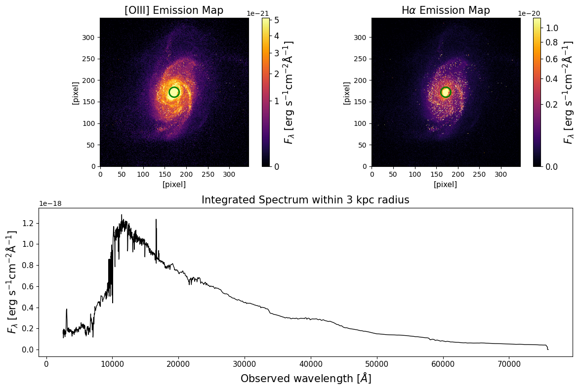
Next, we check spectrum integrated within a circular aperture around the galaxy’s center along with maps of [OIII] and \(\text{H}_{\alpha}\).

import matplotlib.gridspec as gridspec
import matplotlib.patches as patches
import matplotlib.cm as cm
import numpy as np

sci_data = cube['OBS_SPEC_DUST'].data
wavelength = cube['WAVELENGTH_GRID'].data['WAVELENGTH']

pix_kpc = cube[0].header['pix_kpc']
radius_kpc = 3.0
radius_pixels = radius_kpc / pix_kpc

# Select wavelength grids around the OIII and H-alpha lines
oiii_wave_range = [5007*(1.0+z)-100, 5007*(1.0+z)+100]
halpha_wave_range = [6564*(1.0+z)-100, 6564*(1.0+z)+100]
oiii_indices = np.where((wavelength >= oiii_wave_range[0]) & (wavelength <= oiii_wave_range[1]))[0]
halpha_indices = np.where((wavelength >= halpha_wave_range[0]) & (wavelength <= halpha_wave_range[1]))[0]

# Integrate to get the 2D maps
oiii_map = np.sum(sci_data[oiii_indices, :, :], axis=0)
halpha_map = np.sum(sci_data[halpha_indices, :, :], axis=0)

# Get the spatial dimensions
nz, ny, nx = sci_data.shape
center_x, center_y = (nx-1.0)/2.0, (ny-1.0)/2.0

# Create a circular mask
y, x = np.ogrid[:ny, :nx]
dist_from_center = np.sqrt((x - center_x)**2 + (y - center_y)**2)
mask = dist_from_center <= radius_pixels

# Create masked data cube
masked_sci_data0 = sci_data * mask

# Integrated spectrum
integrated_spectrum0 = np.sum(masked_sci_data0, axis=(1, 2))

# Create the multipanel plot
plt.figure(figsize=(12, 8))
gs = gridspec.GridSpec(2, 2, width_ratios=[1, 1], height_ratios=[1, 1])

# OIII map
ax0 = plt.subplot(gs[0, 0])

cmap = cm.get_cmap('inferno').copy()
cmap.set_bad(color='black')
norm = simple_norm(oiii_map, 'sqrt', percent=98.5)
im0 = ax0.imshow(oiii_map, norm=norm, origin='lower', cmap=cmap)

ax0.set_title('[OIII] Emission Map', fontsize=15)
ax0.set_xlabel('[pixel]', fontsize=11)
ax0.set_ylabel('[pixel]', fontsize=11)
#plt.colorbar(im0, ax=ax0, label='Integrated Flux')

cbar = plt.colorbar(im0, ax=ax0)
cbar.set_label(r'$F_{\lambda}$ [erg $\rm{s}^{-1}\rm{cm}^{-2}\AA^{-1}$]', fontsize=15)
cbar.ax.tick_params(labelsize=12)

# New code to add circle to OIII map
circle0 = patches.Circle((center_x, center_y), radius_pixels, edgecolor='green', facecolor='none', linewidth=2)
ax0.add_patch(circle0)
# End of new code

# H-alpha map
ax1 = plt.subplot(gs[0, 1])

cmap = cm.get_cmap('inferno').copy()
cmap.set_bad(color='black')
norm = simple_norm(halpha_map, 'sqrt', percent=98.5)
im1 = ax1.imshow(halpha_map, norm=norm, origin='lower', cmap=cmap)

ax1.set_title(r'H$\alpha$ Emission Map', fontsize=15)
ax1.set_xlabel('[pixel]', fontsize=11)
ax1.set_ylabel('[pixel]', fontsize=11)

cbar = plt.colorbar(im1, ax=ax1)
cbar.set_label(r'$F_{\lambda}$ [erg $\rm{s}^{-1}\rm{cm}^{-2}\AA^{-1}$]', fontsize=15)
cbar.ax.tick_params(labelsize=12)

# New code to add circle to H-alpha map
circle1 = patches.Circle((center_x, center_y), radius_pixels, edgecolor='green', facecolor='none', linewidth=2)
ax1.add_patch(circle1)
# End of new code

# Integrated spectrum
ax2 = plt.subplot(gs[1, :])
ax2.plot(wavelength, integrated_spectrum0, lw=1, color='black')
ax2.set_title('Integrated Spectrum within 3 kpc radius', fontsize=15)
ax2.set_xlabel(r'Observed wavelength [$\AA$]', fontsize=15)
ax2.set_ylabel(r'$F_{\lambda}$ [erg $\rm{s}^{-1}\rm{cm}^{-2}\AA^{-1}$]', fontsize=15)
plt.setp(ax2.get_yticklabels(), fontsize=11)
plt.setp(ax2.get_xticklabels(), fontsize=11)

plt.tight_layout()
plt.show()