Simulating the Observational Effects#
To bridge the gap between theoretical models and observational data, it is essential to add observational effects to synthetic data.
Adding observational effects on synthetic imaging data cube#
The GalSynMockObservation_imaging class in the observe module transforms idealized synthetic images into realistic mock observations.
The process include spatial resapling (to a user-defined pixel scale, matching to the instrument characterictics), PSF convolution, noise simulation and injection.
Please refer Abdurro’uf et al. (2026) for detailed descriptions about the method.
Below, we demonstrate the process of adding observational effects into synthetic images. We will emulate the observational characteristics of the JADES deep imaging observations, specifically the jw011800-deep subregion, as also demonstrated in Abdurro’uf et al. (2026). Please refer to the paper (and reference therein) for more information about the assummed observational characterictics (exposure time, limiting magnitudes, etc.) and how they are obtained. We will use those parameters in the demo below. For the PSFs, we will use empirical PSFs taken from the JADES website.
PSF images used in the following scripts can be found in this online folder.
import numpy as np
from astropy.io import fits
from galsyn import GalSynMockObservation_imaging
from galsyn.utils import make_filter_transmission_text_pixedfit

# select a set of filters to be processed
filters = ['jwst_nircam_f090w', 'jwst_nircam_f115w', 'jwst_nircam_f150w',
            'jwst_nircam_f200w', 'jwst_nircam_f277w', 'jwst_nircam_f335m',
            'jwst_nircam_f356w', 'jwst_nircam_f410m', 'jwst_nircam_f444w']

filter_transmission_path1 = make_filter_transmission_text_pixedfit(filters, output_dir="filters")

# Paths to empirical PSF files
psf_paths = {'jwst_nircam_f090w': 'hlsp_jades_jwst_nircam_jw011800-deep_f090w_v5.0_mpsf.fits',
                'jwst_nircam_f115w': 'hlsp_jades_jwst_nircam_jw011800-deep_f115w_v5.0_mpsf.fits',
                'jwst_nircam_f150w': 'hlsp_jades_jwst_nircam_jw011800-deep_f150w_v5.0_mpsf.fits',
                'jwst_nircam_f200w': 'hlsp_jades_jwst_nircam_jw011800-deep_f200w_v5.0_mpsf.fits',
                'jwst_nircam_f277w': 'hlsp_jades_jwst_nircam_jw011800-deep_f277wa_v5.0_mpsf.fits',
                'jwst_nircam_f335m': 'hlsp_jades_jwst_nircam_jw011800-deep_f335ma_v5.0_mpsf.fits',
                'jwst_nircam_f356w': 'hlsp_jades_jwst_nircam_jw011800-deep_f356wa_v5.0_mpsf.fits',
                'jwst_nircam_f410m': 'hlsp_jades_jwst_nircam_jw011800-deep_f410ma_v5.0_mpsf.fits',
                'jwst_nircam_f444w': 'hlsp_jades_jwst_nircam_jw011800-deep_f444wa_v5.0_mpsf.fits'}

# pixel sizes of the PSF images and exposure times
psf_pixel_scales = {}
exposure_time = {}
for ff in filters:
    psf_pixel_scales[ff] = np.sqrt(fits.open(psf_paths[ff])[0].header['PIXAR_A2'])
    exposure_time[ff] = 87.0 * 60.0 * 60.0        # in seconds

# Below, we define the target depth
# Desired limiting magnitudes to be achieved
# For more information about how these quantities are derived, please see Appendix B in Abdurro'uf et al. (2026)
limiting_magnitude = {'jwst_nircam_f090w': 29.875080925253144,
                        'jwst_nircam_f115w': 30.202076521196858,
                        'jwst_nircam_f150w': 30.120139433909824,
                        'jwst_nircam_f200w': 30.146999402885495,
                        'jwst_nircam_f277w': 31.40929981867027,
                        'jwst_nircam_f335m': 30.822006574170356,
                        'jwst_nircam_f356w': 31.261898835117005,
                        'jwst_nircam_f410m': 30.81580759250037,
                        'jwst_nircam_f444w': 30.997602289188894}
# S/N at the limiting magnitude
snr_limit = {ff: 5.0 for ff in filters}
# aperture radius used in measuring the magnitude limits
aperture_radius_arcsec = {ff: 0.15 for ff in filters}

# desired pixel scale
desired_pixel_scales = {ff: 0.03 for ff in filters}

# Magnitude zero-point, derived from ZPAB = –6.10 – 2.5 log10(PIXAR_SR[sr/pix])
# with PIXAR_SR is pixel area in steradian
mag_zp = {ff: 28.086519392283982 for ff in filters}

# Input idealized data cube
fits_file_path = 'galsyn_39_107965_photo.fits'

# Initialize the mock observation object
simg = GalSynMockObservation_imaging(fits_file_path, filters, psf_paths, psf_pixel_scales, mag_zp,
                                    limiting_magnitude, snr_limit, aperture_radius_arcsec,
                                    exposure_time, filter_transmission_path1, desired_pixel_scales)

# Start the pipeline: Resampling -> PSF Convolution -> Noise Injection
simg.process_images(apply_noise_to_image=True, dust_attenuation=True)

# Save the resulting science and RMS extensions to a new FITS file
output_fits_path = 'obsimg_galsyn_39_107965_photo_30mas.fits'
simg.save_results_to_fits(output_fits_path=output_fits_path)
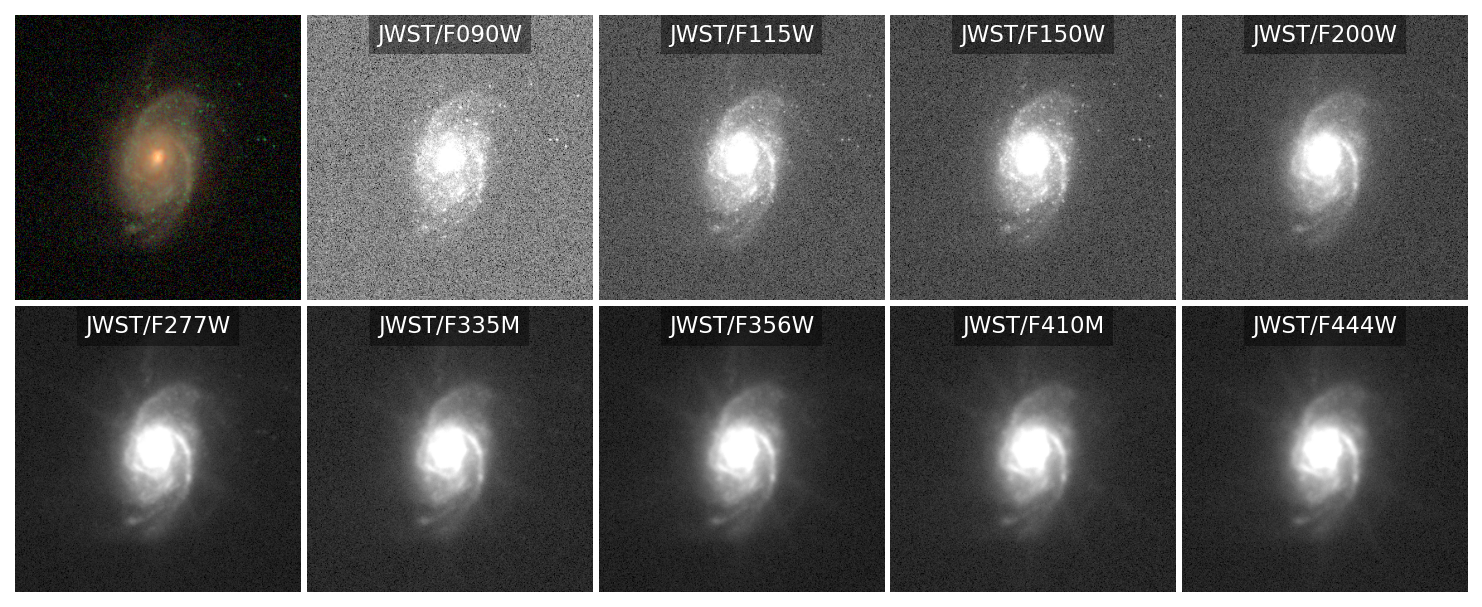
Now, we check the resulting data cube
import matplotlib.pyplot as plt
from astropy.visualization import simple_norm, make_lupton_rgb

# Filter configuration
fils = ['jwst_nircam_f090w', 'jwst_nircam_f115w', 'jwst_nircam_f150w',
            'jwst_nircam_f200w', 'jwst_nircam_f277w', 'jwst_nircam_f335m',
            'jwst_nircam_f356w', 'jwst_nircam_f410m', 'jwst_nircam_f444w']
filnames = ['JWST/F090W', 'JWST/F115W', 'JWST/F150W',
            'JWST/F200W', 'JWST/F277W', 'JWST/F335M',
            'JWST/F356W', 'JWST/F410M', 'JWST/F444W']
nbands = len(fils)

# RGB components (using JWST NIRCam filters)
rgb_fils = ['jwst_nircam_f115w', 'jwst_nircam_f150w', 'jwst_nircam_f200w']

nrows, ncols = 2, 5
fig = plt.figure(figsize=(ncols*2.5, nrows*2.5), dpi=150)

# RGB Composite
ax_rgb = fig.add_subplot(nrows, ncols, 1)
factor = 2e+3

# Access data using the standard 'DUST[FILTER]' extension name
r = cube[f'SCI_DUST_{rgb_fils[2]}'].data * factor
g = cube[f'SCI_DUST_{rgb_fils[1]}'].data * factor
b = cube[f'SCI_DUST_{rgb_fils[0]}'].data * factor

rgb = make_lupton_rgb(r, g, b, stretch=50, Q=10)
ax_rgb.imshow(rgb, origin='lower')
ax_rgb.axis('off') # Cleanly removes all ticks and labels

# Individual Grayscale Bands
for ii in range(nbands):
    ax = fig.add_subplot(nrows, ncols, ii+2)

    # Access dust-attenuated imaging data
    data = cube[f'SCI_DUST_{fils[ii]}'].data

    # Apply square-root normalization to improve dynamic range visibility
    norm = simple_norm(data, 'sqrt', percent=97.5)
    ax.imshow(data, norm=norm, origin='lower', cmap='gray')
    ax.axis('off')

    # Add filter labels with a small background box for readability
    ax.text(0.5, 0.93, filnames[ii], color='white', fontsize=11,
            ha='center', va='center', transform=ax.transAxes,
            bbox=dict(facecolor='black', alpha=0.4, lw=0))

plt.subplots_adjust(hspace=0.02, wspace=0.02)
plt.show()
Adding observational effects on synthetic IFS data cube#
Beyond broadband imaging, GalSyn allows us to simulate realistic Integral Field Unit (IFU) observations. This process transforms idealized spectral cubes into mock IFU observations by accounting for wavelength-dependent sensitivity, instrumental resolution, and spatial blurring.
In this example, we will simulate mock JWST NIRSpec IFU high-resolution data using the G140H/F070LP configuration. There are couple of things we need to prepare for this. First, we will use PSF model generated using the STPSF package and transform it into a standardized format required by GalSyn. Then, we will simulate wavelength-dependent sensitivity limits of the NIRSpec IFU G140H/F070LP instrument configuration using the Pandeia ETC engine. Once we have done all of these, we will run the mock IFU data generation.
The observe module requires a PSF cube where the wavelength axis matches your desired output grid.
Since STPSF outputs multiple extensions, we first extract and standardize the DET_DIST data.
PSF cube used in the following script can be found in this online folder.
import numpy as np
from astropy.io import fits

# The PSF FITS file from STPSF package has multiple extensions.
# We use the DET_DIST extension and store it in a single-extension file.
hdu = fits.open('psf_cube_G140H_F100LP.fits')
psf_cube_data = hdu['DET_DIST'].data

# Extract wavelength information for each slice in the PSF cube
cube_psf_wave_um = np.zeros(psf_cube_data.shape[0])
for i in range(psf_cube_data.shape[0]):
    cube_psf_wave_um[i] = hdu['det_dist'].header["WVLN%04d" % i] * 1e+6
hdu.close()

# Save as a standardized input for GalSyn
hdul = fits.HDUList()
hdul.append(fits.ImageHDU(data=psf_cube_data, name='psf_cube'))
hdul.writeto('psf_G140H_F100LP_standard.fits', overwrite=True)
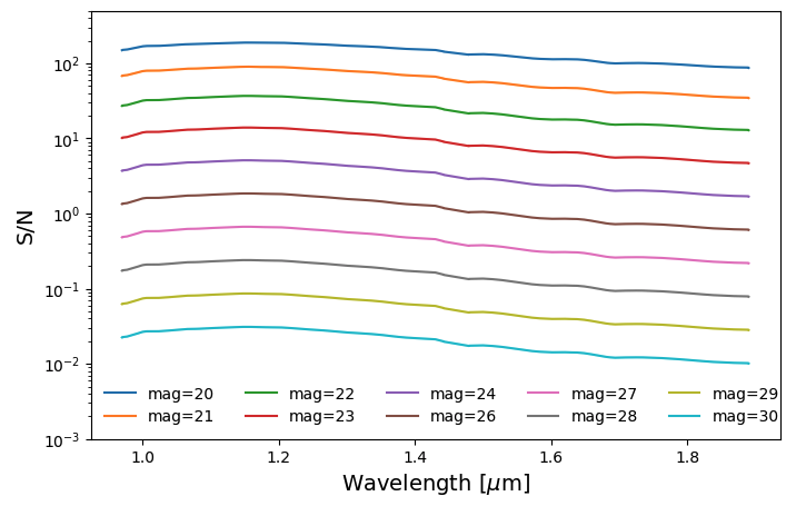
Simulating the NIRSpec IFU sensitiviy using JWST ETC Pandeia Engine#
We will perform S/N simulations using the Pandeia ETC engine to estimate the sensitivity limits of G140H/F070LP. Throughout this experiment, we assume an exposure time of 40 ks. First, we will model a flat input spectrum (i.e.,~constant in AB magnitude) across a grid of source magnitudes ranging from 20 to 30 and input them into the Pandeia ETC engine to estimate the S/N per pixel on the native detector grid.
import warnings
import traceback
from pandeia.engine.calc_utils import build_default_calc
from pandeia.engine.perform_calculation import perform_calculation
from scipy.interpolate import interp1d

def run_nirspec_ifu(wavelengths, fluxes, exposure_time_sec,
                    configs = [{'d': 'g140h',  'f': 'f100lp'}],
                    config_exptimes=None):
    """
    Parameters
    ----------
    wavelengths : array-like
        Wavelength in microns
    fluxes : array-like
        Flux in mJy
    exposure_time_sec : float
        Default exposure time in seconds for all configs
    config_exptimes : dict, optional
        Per-config exposure time overrides. Keys are config names
        (e.g. 'prism/clear', 'g140m/f100lp'). Example:
            config_exptimes = {
                'prism/clear':   1200,
                'g140m/f100lp':  20000,
                'g235m/f170lp':  20000,
                'g395m/f290lp':  20000,
            }

    Returns
    -------
    snr_dict : dict
        Keys are config names, each containing:
            'wave'      : np.ndarray  - wavelength in microns
            'sn'        : np.ndarray  - SNR per pixel
            'scalar_sn' : float       - summary SNR
            'actual_time': float      - actual exposure time used (s)
        For dual-detector configs, 'det1' and 'det2' sub-dicts are used.
    """
    if config_exptimes is None:
        config_exptimes = {}

    calc_input = build_default_calc("jwst", "nirspec", "ifu")

    src = calc_input['scene'][0]
    src['spectrum']['sed'] = {
        'sed_type': 'input',
        'spectrum': (wavelengths.tolist(), fluxes.tolist()),
        'unit': 'mjy',
        'z': 0.0
    }
    src['spectrum']['normalization']['type'] = 'none'

    t_frame = 10.73677

    snr_dict = {}
    success  = False

    for cfg in configs:
        key = f"{cfg['d']}/{cfg['f']}"

        # Use per-config exptime if provided, else fall back to default
        exptime = config_exptimes.get(key, exposure_time_sec)

        #ngroups = max(2, int(round(exptime / t_frame)))
        #actual_time = ngroups * t_frame

        # Instead of making ngroups huge, cap it at 50 and use nint to reach the time
        max_groups_limit = 60  # Stay safely below the 65 limit
        ngroups = max_groups_limit
        nint = max(1, int(round(exptime / (ngroups * t_frame))))

        actual_time = nint * ngroups * t_frame

        calc_input['configuration']['detector'].update({
            'ngroup': ngroups,
            'nint':   nint,   # Use multiple integrations
            'readout_pattern': 'nrs',
            'subarray': 'full'
        })

        try:
            print(f"Calculating {key}  (t = {actual_time:.1f}s)...", end='\r')
            calc_input['configuration']['instrument']['disperser'] = cfg['d']
            calc_input['configuration']['instrument']['filter']    = cfg['f']

            with warnings.catch_warnings():
                warnings.simplefilter("ignore", RuntimeWarning)
                results = perform_calculation(calc_input)

            wave_raw  = np.array(results['1d']['wave_pix'])
            sn_raw    = np.array(results['1d']['sn'])
            scalar_sn = results['scalar']['sn']
            sat_frac  = results['scalar']['fraction_saturation']
            brightest = results['scalar']['brightest_pixel']

            # Warn if saturated
            if brightest > 1.0:
                print(f"\n  {key}: saturated! brightest_pixel={brightest:.2f}, "
                    f"sat_fraction={sat_frac:.3f} — consider reducing exptime.")
            else:
                print(f"  {key:20s}: scalar SNR = {scalar_sn:.1f},  "
                    f"t = {actual_time:.1f}s,  "
                    f"brightest_pixel = {brightest:.3f}")

            def _store_and_plot(w, s, label, det_dict):
                valid = np.isfinite(s) & (s > 0)
                if valid.any():
                    det_dict['wave'] = w[valid]
                    det_dict['sn']   = s[valid]

            if wave_raw.ndim == 2 and sn_raw.ndim == 2:
                snr_dict[key] = {'scalar_sn': scalar_sn, 'actual_time': actual_time}
                for i in range(wave_raw.shape[0]):
                    det = {}
                    _store_and_plot(wave_raw[i], sn_raw[i], f"{key} det{i+1}", det)
                    snr_dict[key][f'det{i+1}'] = det

            elif wave_raw.ndim == 1 and sn_raw.ndim == 2:
                snr_dict[key] = {'scalar_sn': scalar_sn, 'actual_time': actual_time}
                for i in range(sn_raw.shape[0]):
                    det = {}
                    _store_and_plot(wave_raw, sn_raw[i], f"{key} det{i+1}", det)
                    snr_dict[key][f'det{i+1}'] = det

            else:
                wave  = wave_raw.flatten()
                sn    = sn_raw.flatten()
                valid = np.isfinite(sn) & (sn > 0)
                snr_dict[key] = {
                    'wave':       wave[valid],
                    'sn':         sn[valid],
                    'scalar_sn':  scalar_sn,
                    'actual_time': actual_time
                }

            success = True

        except Exception:
            traceback.print_exc()

    return snr_dict

def calculate_sensitivity_limits(snr_results, target_snr=5.0):
    # Define "Common Grids" for NIRSpec IFU modes (microns)
    # These represent the standard operational ranges for each disperser
    common_grids = {
        'prism':  np.linspace(0.6, 5.3, 500),
        'g140m':  np.linspace(0.7, 1.9, 500),
        'g235m':  np.linspace(1.6, 3.2, 500),
        'g395m':  np.linspace(2.8, 5.3, 500),
        'g140h':  np.linspace(0.7, 1.9, 1000),
        'g235h':  np.linspace(1.6, 3.2, 1000),
        'g395h':  np.linspace(2.8, 5.3, 1000)
    }

    sensitivity_dict = {}

    mags = list(snr_results.keys())
    configs = list(snr_results[mags[0]].keys())

    for config in configs:
        disperser = config.split('/')[0].lower()
        target_grid = common_grids.get(disperser, np.linspace(0.6, 5.3, 500))

        # Prepare sub-dictionary for detectors
        sensitivity_dict[config] = {'common_wave': target_grid}

        # Determine if we have det1/det2 or just a single array
        sub_keys = ['det1', 'det2'] if 'det1' in snr_results[mags[0]][config] else ['main']

        for sk in sub_keys:
            snr_stack = []
            native_waves = None

            # Extract SNR across all magnitudes
            for m in mags:
                data = snr_results[m][config]
                d = data[sk] if sk != 'main' else data
                native_waves = d['wave']
                snr_stack.append(d['sn'])

            snr_stack = np.array(snr_stack)

            # Interpolate each magnitude's SNR onto the common wavelength grid first
            # Then interpolate to find the Mag where SNR=5
            interp_mags = np.zeros_like(target_grid)

            for i, w_target in enumerate(target_grid):
                # Find SNR at this specific wavelength for all magnitudes
                sn_at_w = []
                for s_array in snr_stack:
                    # Linear interp of SNR vs Wavelength
                    val = np.interp(w_target, native_waves, s_array, left=0, right=0)
                    sn_at_w.append(val)

                sn_at_w = np.array(sn_at_w)

                # Now solve for Mag where SNR=5 (using Log10 for linearity)
                if np.any(sn_at_w >= target_snr) and np.any(sn_at_w > 0):
                    mask = sn_at_w > 0
                    f_mag = interp1d(np.log10(sn_at_w[mask]), np.array(mags)[mask],
                                        kind='linear', fill_value="extrapolate")
                    interp_mags[i] = f_mag(np.log10(target_snr))
                else:
                    interp_mags[i] = np.nan

            sensitivity_dict[config][sk] = interp_mags

    return sensitivity_dict


# Run the simulation using the function
exptime = 40000
magnitudes = np.linspace(20.0, 30.0, 10)

# Define wavelength grid (microns)
waves = np.linspace(0.6, 5.3, 500)

# Dictionary to store all results
# Structure: results[magnitude] = snr_dict
snr_results = {}

for mag in magnitudes:
    # 2. Calculate flux in mJy for a flat AB magnitude spectrum
    # Formula: m_ab = -2.5 * log10(f_nu_Jy / 3631)
    # So: f_nu_mJy = 3631 * 10^(-mag / 2.5) * 10^3
    flux_mjy_val = 3631 * 10**(-mag / 2.5) * 1e3
    fluxes = np.ones_like(waves) * flux_mjy_val

    # 3. Run the Pandeia engine function
    # Note: We pass exptime as the third argument (exposure_time_sec)
    snr_dict = run_nirspec_ifu(waves, fluxes, exptime)

    # Store result
    snr_results[mag] = snr_dict

# plotting
import matplotlib.pyplot as plt

fig = plt.figure(figsize=(8,5))
f1 = plt.subplot()
f1.set_yscale('log')
plt.xlabel(r'Wavelength [$\mu$m]', fontsize=14)
plt.ylabel('S/N', fontsize=14)
plt.ylim(1e-3,5e+2)

for mag in magnitudes:
    plt.plot(snr_results[mag]['g140h/f100lp']['det2']['wave'], snr_results[mag]['g140h/f100lp']['det2']['sn'], label='mag=%.0lf' % mag)

plt.legend(fontsize=10, frameon=False, ncol=5)
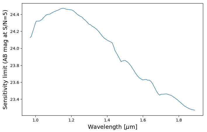
Then we will use the derived S/N curves to estimate the magnitude limits at S/N=5 across the wavelength grids.
sensitivity_dict = calculate_sensitivity_limits(snr_results, target_snr=5.0)
sensitivity_wave = sensitivity_dict['g140h/f100lp']['common_wave']
sensitivity_mag_lims = sensitivity_dict['g140h/f100lp']['det2']

fig = plt.figure(figsize=(8,5))
f1 = plt.subplot()
#f1.set_yscale('log')
plt.xlabel(r'Wavelength [$\mu$m]', fontsize=14)
plt.ylabel('Sensitivity limit (AB mag at S/N=5)', fontsize=14)

plt.plot(sensitivity_wave, sensitivity_mag_lims, lw=1)
The GalSynMockObservation_ifu module processes the data through a specific sequence designed for 3D spectroscopic data:
Spectral Grid Alignment: The high-resolution synthetic cube is interpolated onto your
desired_wave_grid.Spatial Resampling: The cube is resampled to the
final_pixel_scale_arcsecwhile maintaining flux conservation.Spectral Smoothing: Each spaxel is convolved along the wavelength axis with a Gaussian kernel to match the target instrumental resolution (\(R\)).
Spatial PSF Convolution: The cube is convolved slice-by-slice using the 3D PSF cube to account for wavelength-dependent blurring.
Noise Injection: Realistic, wavelength-dependent noise is injected independently into each slice.
Additional notes:
Wavelength-dependent parameters: unlike imaging, parameters like
limiting_magnitudeandexposure_timecan be provided as functions of wavelength to model instrument sensitivity variations accurately.Spectral smoothing: the module uses your
spectral_resolution_Rto derive the kernel width (\(\sigma = \lambda / R / 2.355\)) for each wavelength channel.
from scipy.interpolate import interp1d
from galsyn import GalSynMockObservation_ifu


fits_file_path = 'galsyn_39_107965_specphoto.fits'
desired_wave_grid = cube_psf_wave_um * 1e+4  # Convert microns to Angstroms
psf_cube_path = 'psf_G140H_F100LP_standard.fits'

# Observation parameters
psf_pixel_scale = 0.1
spectral_resolution_R = 2700
mag_zp = 25.472125665882295
exposure_time = 40000
final_pixel_scale_arcsec = 0.1

# Define a wavelength-dependent limiting magnitude function
limiting_magnitude_wave_func = interp1d(sensitivity_wave * 1e+4, sensitivity_mag_lims, fill_value="extrapolate")
snr_limit = 5.0

# Initialize and run the IFU pipeline
sifu = GalSynMockObservation_ifu(fits_file_path, desired_wave_grid, psf_cube_path, psf_pixel_scale,
                spectral_resolution_R, mag_zp, limiting_magnitude_wave_func, snr_limit,
                final_pixel_scale_arcsec, exposure_time)

sifu.process_datacube(dust_attenuation=True, apply_noise_to_cube=True)

# Save the final realistic IFU data cube
output_fits_path = 'obsifu_nirspec_g140h_f100lp_galsyn_39_107965_100mas.fits'
sifu.save_results_to_fits(output_fits_path)
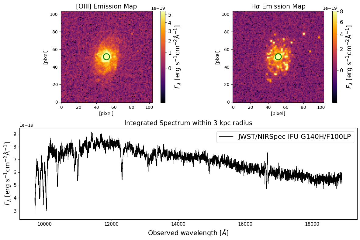
Let’s check the output data cube.
import matplotlib.pyplot as plt
from astropy.visualization import simple_norm
import matplotlib.gridspec as gridspec
import matplotlib.patches as patches
import matplotlib.cm as cm
from astropy.cosmology import Planck18 as cosmo
import astropy.units as u

cube = fits.open('obsifu_nirspec_g140h_f100lp_galsyn_39_107965_100mas.fits')

sci_data = cube['SCI_DUST'].data
wavelength = cube['WAVELENGTH_GRID'].data['WAVELENGTH']

# get physical scale of pixel in kpc
z = 1.531239    # redshift
kpc_per_arcsec = 1.0 / cosmo.arcsec_per_kpc_proper(z).value
pix_kpc = cube[0].header['pixsize'] * kpc_per_arcsec
print (f'physical scale of pixel: {pix_kpc} kpc')
radius_kpc = 3.0
radius_pixels = radius_kpc / pix_kpc

# Select wavelength grids around the OIII and H-alpha lines
oiii_wave_range = [5007*(1.0+z)-200, 5007*(1.0+z)+200]
halpha_wave_range = [6564*(1.0+z)-200, 6564*(1.0+z)+200]
oiii_indices = np.where((wavelength >= oiii_wave_range[0]) & (wavelength <= oiii_wave_range[1]))[0]
halpha_indices = np.where((wavelength >= halpha_wave_range[0]) & (wavelength <= halpha_wave_range[1]))[0]

# Integrate to get the 2D maps
oiii_map = np.sum(sci_data[oiii_indices, :, :], axis=0)
halpha_map = np.sum(sci_data[halpha_indices, :, :], axis=0)

# Get the spatial dimensions
nz, ny, nx = sci_data.shape
center_x, center_y = (nx-1.0)/2.0, (ny-1.0)/2.0

# Create a circular mask
y, x = np.ogrid[:ny, :nx]
dist_from_center = np.sqrt((x - center_x)**2 + (y - center_y)**2)
mask = dist_from_center <= radius_pixels

# Create masked data cube
masked_sci_data0 = sci_data * mask

# Integrated spectrum
integrated_spectrum0 = np.sum(masked_sci_data0, axis=(1, 2))

# Create the multipanel plot
plt.figure(figsize=(12, 8))
gs = gridspec.GridSpec(2, 2, width_ratios=[1, 1], height_ratios=[1, 1])

# OIII map
ax0 = plt.subplot(gs[0, 0])

cmap = cm.get_cmap('inferno').copy()
cmap.set_bad(color='black')
norm = simple_norm(oiii_map, 'sqrt', percent=98.5)
im0 = ax0.imshow(oiii_map, norm=norm, origin='lower', cmap=cmap)

ax0.set_title('[OIII] Emission Map', fontsize=15)
ax0.set_xlabel('[pixel]', fontsize=11)
ax0.set_ylabel('[pixel]', fontsize=11)
#plt.colorbar(im0, ax=ax0, label='Integrated Flux')

cbar = plt.colorbar(im0, ax=ax0)
cbar.set_label(r'$F_{\lambda}$ [erg $\rm{s}^{-1}\rm{cm}^{-2}\AA^{-1}$]', fontsize=15)
cbar.ax.tick_params(labelsize=12)

# New code to add circle to OIII map
circle0 = patches.Circle((center_x, center_y), radius_pixels, edgecolor='green', facecolor='none', linewidth=2)
ax0.add_patch(circle0)
# End of new code

# H-alpha map
ax1 = plt.subplot(gs[0, 1])

cmap = cm.get_cmap('inferno').copy()
cmap.set_bad(color='black')
norm = simple_norm(halpha_map, 'sqrt', percent=98.5)
im1 = ax1.imshow(halpha_map, norm=norm, origin='lower', cmap=cmap)

ax1.set_title(r'H$\alpha$ Emission Map', fontsize=15)
ax1.set_xlabel('[pixel]', fontsize=11)
ax1.set_ylabel('[pixel]', fontsize=11)

cbar = plt.colorbar(im1, ax=ax1)
cbar.set_label(r'$F_{\lambda}$ [erg $\rm{s}^{-1}\rm{cm}^{-2}\AA^{-1}$]', fontsize=15)
cbar.ax.tick_params(labelsize=12)

# New code to add circle to H-alpha map
circle1 = patches.Circle((center_x, center_y), radius_pixels, edgecolor='green', facecolor='none', linewidth=2)
ax1.add_patch(circle1)
# End of new code

# Integrated spectrum
ax2 = plt.subplot(gs[1, :])
ax2.plot(wavelength, integrated_spectrum0, lw=1, color='black')
ax2.set_title('Integrated Spectrum within 3 kpc radius', fontsize=15)
ax2.set_xlabel(r'Observed wavelength [$\AA$]', fontsize=15)
ax2.set_ylabel(r'$F_{\lambda}$ [erg $\rm{s}^{-1}\rm{cm}^{-2}\AA^{-1}$]', fontsize=15)
plt.setp(ax2.get_yticklabels(), fontsize=11)
plt.setp(ax2.get_xticklabels(), fontsize=11)

plt.tight_layout()